Exploring Meta-learned Curiosity Algorithms
This blog post delves into Alet et al.'s ICLR 2020 paper, Meta-learning curiosity algorithms, which introduces a unique approach to meta-learning curiosity algorithms. Instead of meta-learning neural network weights, the focus is on meta-learning pieces of code, allowing it to be interpretable by humans. The post explores the two meta-learned algorithms, namely Fast Action Space Transition (FAST) and Cycle-Consistency Intrinsic Motivation (CCIM).
Introduction
Dealing with environments with sparse rewards, i.e., feedback comes at a low frequency, in reinforcement learning (RL) requires meaningful exploration. One way to encourage the RL agent to perform meaningful exploration is by instilling intrinsic motivation into the agents. This intrinsic motivation usually comes in the form of curiosity. As Schmidhuber
Now there has been success with curious agents solving environments with sparse rewards
The roadmap for exploring FAST and CCIM is organised as follows. We begin with a brief introduction to RL, meta-learning, and meta-reinforcement learning (meta-RL). Next, we provide concise explanations of how curiosity-driven exploration baselines, RND and BYOL-Explore, operate. Subsequently, we delve into the discovery process of FAST and CCIM. Following that, we explore the intricacies of FAST and CCIM, evaluating their performance and studying their behaviour in both the empty grid-world environment and the bsuite deep sea environment. We then compare them to curiosity-driven baselines and a non-curious agent. Finally, we conclude our journey.
Background
Reinforcement Learning
RL is inspired by how biological systems learn as animals are to able learn through trial-and-error. In RL we have an agent that tries to maximise the sum of rewards it recieves by learning from its interactions with the environment. This agent-environment interaction is usually modelled as a Markov decision process (MDP). Figure 1 below illstrustates this agent-environment interaction.
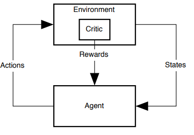
From the figure we can see that the agent observes a state and then takes action. The agent can then decide on its next action based on the next state it observes and the rewards it receives from the critic in the environment. The critic decides on what reward the agent receives at every time-step by evaluating its behaviour.
As Sutton et al. highlighted in
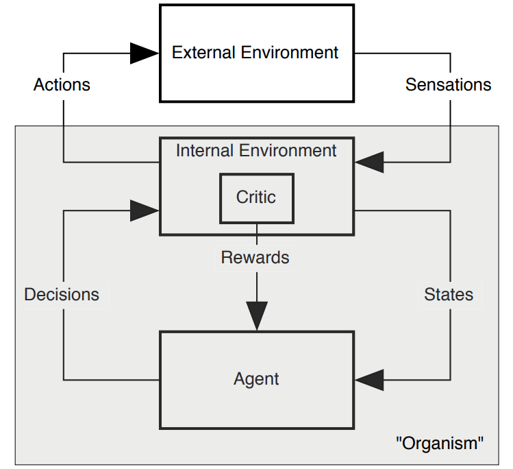
Singh et al. highlighted in
Meta-RL and Meta-learning
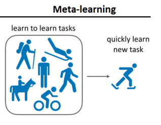
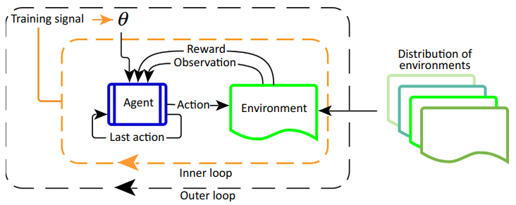
The next stop on our journey takes us to meta-learning. Meta-learning is about learning how to to learn. The goal is for meta-learning agents to enhance their learning abilities over time, enabling them to generalise to new, unseen tasks. Meta-learning involves two essential loops: the inner loop and the outer loop. In the inner loop, our learning algorithm adapts to a new task using experiences obtained from solving other tasks in the outer loop, which is referred to as meta-training
The inner loop addresses a single task, while the outer loop deals with the distribution of tasks. Figure 3 illustrates this concept of meta-learning.
Moving into the intersection of meta-learning and reinforcement learning (RL) is meta-RL, where the agent learns how to reinforcement learn
In basic RL, we have an algorithm \(f\) that outputs a policy, mapping states to actions. However, in meta-RL, our algorithm has meta-parameters \(\theta\) that outputs \(f\), and \(f\) then produces a policy when faced with a new MDP. Figure 4 illustrates that the meta-RL process. Note that in the outer loop the meta-parameters \(\theta\) are updated.
Random Network Distillation
We now move onto our curiosity-driven exploration baselines. The first baseline that we will briefly discuss is RND
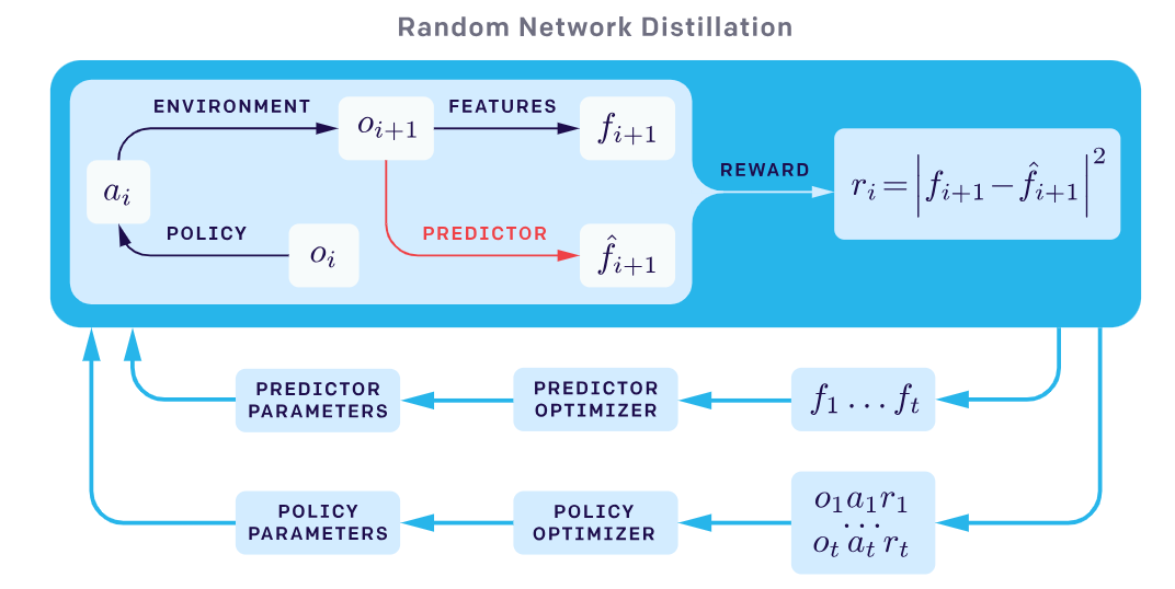
where \(\hat{f}_t\) is the output of the predictor network. The formula above also serves as the loss function of the predictor network. We normalise \(r_i\) by dividing it by the running estimate of the standard deviations of the intrinsic returns. We do this because the intrinsic rewards can be very different in various environments. Normalising the intrinsic rewards make it easier to pick hyperparameters that work across a wide range of environments. As the agent explores more the predictor network will get better and the intrinsic rewards will decrease. The key idea in RND is that the predictor network is trying to predict the output of a network that is deterministic, the target network. The figure below illustrates the process of RND.
BYOL-Explore
BYOL-Explore builds upon Bootstrap Your Own Latent (BYOL)
In the above equation, \(\phi\), is the target network’s parameters, \(\theta\) is the online network’s predictor parameters and \(\alpha\) is the EMA smoothing factor. In our implementation of BYOL-Explore we do not make use of the RNN cells as we are dealing with simple environments, we call our implementation BYOL-Explore Lite. In our implementation the online network is composed of a multilayer perceptron (MLP) encoder and a predictor. The target network, \(h\), is just composed of an MLP encoder. In the BYOL-Explore Lite process the current state of the environment, \(s_t\), is inputted into the encoder \(f\), which outputs a feature representation of the state, \(f(s_t)\). This feature representation is then passed to both the RL agent and the predictor \(g\). The RL agent uses \(f(s_t)\) to decide on its next action and determine the value of that state. The predictor uses \(f(s_t)\) to predict \(h(s_{t+1})\), i.e., the predictor is attempting to predict the target network’s output for the next state. There are two losses namely the encoder loss and the predictor loss. The predictor loss is given by,
\[\mathcal{L}_p=\left\|\frac{g(f(s_{t}))}{\|g(f(s_{t}))\|_2}-\frac{h(s_{t+1})}{\|h(s_{t+1})\|_2}\right\|_2^2.\]Since the RL agent and the predictor both make use of the online network’s encoder its loss is given by the sum of the RL loss and the predictor loss. Importantly, the loss \(\mathcal{L}_p\) serves as the intrinsic reward that the RL agent receives at each step. We normalise the intrinsic rewards by dividing it by the EMA estimate of their standard deviation.
BYOL-Explore Lite also makes use of something known as reward prioritisation. Reward prioritisation involves focusing on parts of the environment where the agent receives high intrinsic rewards while disregarding those with low intrinsic rewards. This enables the agent to concentrate on areas it understands the least. Over time the previously ignored areas with low intrinsic rewards become the priority for the agent. To do this we take the EMA mean relative to the successive batch of normalised intrinsic rewards, $\mu$. Note that $\mu$ is used as a threshold to separate the high intrinsic rewards and the low intrinsic rewards. Therefore, the intrinsic rewards that agent obtains after reward prioritisation is,
\[i_t=\max(ri_t-\mu,\,0),\]where $ri_t$ is the normalised intrinsic reward.
Meta-learning curiosity algorithms
Alet et al.
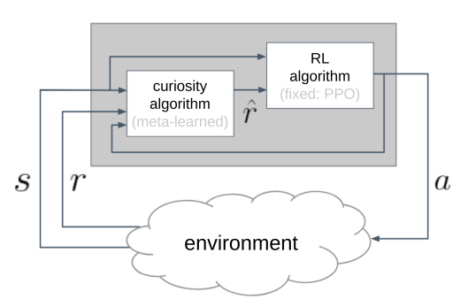
In the above figure we can see that the curiosity algorithm, \(\mathcal{C}\), takes in the state and reward from the environment and then feeds proxy reward \(\hat{r}\) to the RL agent. The RL algorithm used is a fully-specified algorithm, i.e., all its hyperparameters are specified. There were two stages in the authors search because the module \(\mathcal{C}\) is made of two components. The first component, \(\mathcal{I}\), calculates the intrinsic reward given the current state, next state and the action taken. The second component, \(\chi\), then takes the extrinsic reward, the intrinsic reward and the current normalised time step to combine them and output \(\hat{r}\).
Meta-Learned Components and their DAGs
As mention earlier Alet et al. focused on meta-learning pieces of code or rather meta-learning in a space of programs or operations. The programs and operations are represented in a domain-specific language (DSL). The DSL used to find component \(\chi\) consisted of operations such as arithmetic, Min, Max and more. While the DSL used to find component \(\mathcal{I}\) consisted of programs such as neural networks complete with gradient-descent mechanisms, L2 distance calculation, and ensembles of neural networks and more. Component \(\mathcal{I}\)’s DSL can describe many other hand-designed curiosity algorithms in literature, such as RND.
The components \(\mathcal{I}\) and \(\chi\) are represented as Directed Acyclic Graphs (DAGs). The DAGs consist of the following types of modules:
- Input modules: These are the inputs we put in each component of module \(\mathcal{C}\).
- Parameter and Buffer modules: This module either consists of the weights of a neural network which can be updated via back-propagation or First In, First Out queues that output a finite list of the most recent \(k\) inputs.
- Functional modules: This type of module calculates the output given some input.
- Update modules: These modules can add real-valued outputs to the loss function of the neural network or add variables to buffers.
The DAGs also have an output node which is a single node and the output of this node is the output of the entire program. To make these ideas more concrete, let us look the DAG that describes RND.
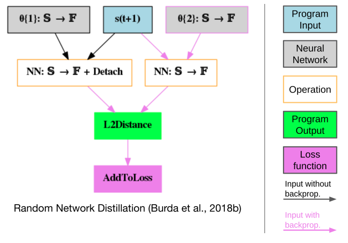
The blue rectangles represent the input modules, and we can see from the figure that the inputs are states from the environment. The parameter modules are the gray rectangles and these are the parameters of the target network and the predictor network. Note that the target network’s parameters are given by \(\theta\){1} and the predictor network’s parameter’s are given by \(\theta\){2}. The functional modules are the white rectangles and these are the neural networks. The update module is the pink rectangle which is the loss function.
The output node is the green rectangle and is the L2 distance between the output of predictor network and the target network. This is the loss function described in the RND section. Note that the \(\theta\){2} rectangle has a pink border and a pink arrow, this indicates that it can be updated via back-propagation. While the \(\theta\){1} rectangle has black border and a black arrow indicating the parameters are not updated via back-propagation. Also note that the functional module that makes use of those parameters has the word “Detach” indicating the gradient information is not flowing back. Recall that \(\theta\){1} represents the parameters of the target network, which remain fixed, and \(\theta\){2} represents the parameters of the predictor network, which are updated during training.
Now a very important idea is that the DAGs used in the paper have polymorphic types for the inputs and outputs. There are four types:
- \(\mathbb{R}\), the real numbers.
- \(\mathbb{S}\), the state space of the environment.
- \(\mathbb{A}\), the action space of the environment.
- \(\mathbb{F}\), the feature space.
The instantiation of some types depends on the environment. For example in Figure 7, if \(\mathbb{S}\) is an image then both the target network and the predictor network are instantiated as a convolutional neural network. If \(\mathbb{S}\) is just an array of numbers then target network and the predictor network are fully connected neural networks. We now look at the method used to find the components \(\mathcal{I}\) and \(\chi\).
Method
We now turn our attention to how component \(\mathcal{I}\) was searched for. Alet et al. decided to focus on environment that has sparse rewards. They chose an image-based grid-world. In this environment the agent is tasked with finding the goal position and only obtains a reward if it finds the goal position. This environment has sparse rewards as the agent only receives feedback once it finds the goal position. They limited the number of operations that component \(\mathcal{I}\) could perform to 7 so that the search space remains manageable, and we can still interpret the algorithm. They focused on finding a component \(\mathcal{I}\) that optimises the number of distinct cells visited. From the search 13 of the top 16 components found where variants of FAST and 3 of them were variants of CCIM. We will cover FAST and CCIM in the upcoming sections.
For the component \(\chi\) they focused on the Lunar Lander environment as it has a strong external reward signal. The algorithm used to output the intrinsic reward was a variant of RND. The main difference was that instead of single neural network for the predicator network an ensemble is used. This algorithm came from a preliminary set of algorithms that all resemble RND. The best reward combiner found was,
\[\hat{r}_t = \frac{(1+ri_t-t/T)\cdot ri_t+ r_t\cdot t/T}{1+ri_t}.\]Here \(r_t\) is the external reward, \(t\) is the current time-step, \(T\) is the maximum steps possible in the episode, and \(ri_t\) is the intrinsic reward. However, in this blog post we decided not to focus on the reward combiner \(\chi\) but instead focus on FAST and CCIM.
FAST
FAST is very simple algorithm in that it only contains one neural network. Below is the DAG of FAST.
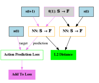
This single neural network in FAST is a policy-mimicking network, \(\hat{\pi}\). The network \(\hat{\pi}\) tries to predict what action the agent took given a state of the environment
This is different from RND and BYOL-Explore Lite. The intrinsic reward is not given by a predictive error or the loss function of one of the networks in the program. We understood the above formula as the L2 difference between the logits of the current state and the next state. The agent is then rewarded if the next state’s logits is different from the current state. Importantly, the agent isn’t rewarded for taking a different action in the next state. Alet et al. pointed out that if the policy-mimicking network has a uniform distribution over the action space in all states, the agent will receive an intrinsic reward of zero. Therefore, in environments where the action probability distributions outputted by the policy-mimicking network vary across states, we expect this algorithm to generate intrinsic rewards. We hypothesize that this algorithm may not perform well in environments where the optimal policy requires the agent to visit states with very similar action probability distributions. While the agent explores by going to different states, ideally, we wish for the intrinsic rewards to decrease as the agent explores. Looking at the output of FAST it is not clear to use how the intrinsic reward decreases, and we expect that this could cause issues.
CCIM
CCIM took us quite a while to understand and process. Let us first go through its DAG below.
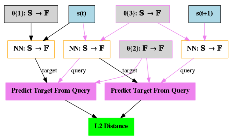
We can see that there are 3 neural networks: a random network, a random and forward network, and a backward network. The parameters \(\theta\){1} are the parameters of the random network, \(\theta\){2} are the parameters of the backward network, and \(\theta\){3} are the parameters of the random and forward network. Looking at the black border of \(\theta\){1}’s rectangle we can see that the random network’s parameters stay fixed during training like in RND. Let us denote the random network as \(r_{\theta_1}\), the backward network as \(b_{\theta_2}\), and the random and forward network as \(fr_{\theta_3}\). Let us look at the loss function of the \(b_{\theta_2}\) and \(fr_{\theta_3}\). The loss function of \(b_{\theta_2}\) is given by,
\[\mathcal{L}_b=\|b_{\theta_2}(fr_{\theta_3}(s_t))-r_{\theta_1}\|_2+\|b_{\theta_2}(fr_{\theta_3}(s_{t+1}))-fr_{\theta_3}(s_t)\|_2,\]and the loss function for \(fr_{\theta_3}\) is
\[\mathcal{L}_f=\|b_{\theta_2}(fr_{\theta_3}(s_t))-r_{\theta_1}\|_2.\]Note the first term in \(\mathcal{L}_b\) is the same as \(\mathcal{L}_f\). The intrinsic reward, i.e., the output of this program is given by,
\[ri_t=\|b_{\theta_2}(fr_{\theta_3}(s_{t+1}))-b_{\theta_2}(fr_{\theta_3}(s_t))\|_2.\]Looking at the equations, we can see that CCIM borrows ideas from the cycle-consistency seen in the Image-to-Image Translation literature. The cycle-consistency ensures that if you translate from space \(A\) to space \(B\), then given space \(B\), you should be able to translate back to space \(A\). To see how CCIM applies this, let us turn our attention to \(\mathcal{L}_f\)’s equation. The \(fr_{\theta_3}\) network applies a random embedding to state \(s_t\). It then forwards this random embedding to the “next state”. The \(b_{\theta_2}\) network then takes this forwarded random embedding of state \(s_t\) and undoes the forward transformation so that we end up again with just the random embedding of state \(s_t\). Now, the random embedding that \(fr_{\theta_3}\) applied should match the random embedding that \(r_{\theta_1}\) applied to the state \(s_t\) for the loss to be minimised. In other words, once we apply a forward transformation to the random embedding of the state, we should be able to undo that transformation and end up where we started.
Let us look at the second term in \(\mathcal{L}_b\) given by \(\|b_{\theta_2}(fr_{\theta_3}(s_{t+1}))-fr_{\theta_3}(s_t)\|_2\). We apply a forward and then a backward transformation to the random embedding of state \(s_{t+1}\), so we should end up with just the random embedding of state \(s_{t+1}\). We then apply \(fr_{\theta_3}\) to state \(s_t\) and end up with the forwarded random embedding of state \(s_t\), which should equal the random embedding of \(s_{t+1}\).
The intrinsic reward confuses us. Looking at the DAG of CCIM, we see that the output is given by the L2 distance between \(\mathcal{L}_f\) and \(\mathcal{L}_b\); hence, we initially thought the intrinsic reward was given by \(\|b_{\theta_2}(fr_{\theta_3}(s_{t+1}))-fr_{\theta_3}(s_t)\|\). The difference between this equation and the original intrinsic reward equation is that the backward model, \(b_{\theta_2}\), is not applied to the \(fr_{\theta_3}(s_t)\) term. Looking at the original formula of the intrinsic reward, we can see that it is just the difference between the random embedding of the current state and the next state
CCIM-slimmed
Through our communication with them, Alet et al. recommended we try ablations of CCIM and they suggested the following slimmed-down version of CCIM:
- Network \(r_{\theta_1}\) remains unchanged and its parameters stay fixed.
- Network \(fr_{\theta_3}\) changes to just being a forward network, \(f_{\theta_3}\).
- The loss function of the \(f_{\theta_3}\) is now \(\mathcal{L}_f=\|f_{\theta_3}(r_{\theta_1}(s_t))-r_{\theta_1}(s_{t+1})\|_2^2\).
- Network \(b_{\theta_2}\)’s loss function, \(\mathcal{L}_b\), also changes. \(\mathcal{L}_b=\|b_{\theta_2}(r_{\theta_1}(s_{t+1}))-r_{\theta_1}(s_{t})\|_2^2\).
- The intrinsic reward is now \(\mathcal{L}_f+\mathcal{L}_b\).
This slimmed down version of CCIM was much easier to implement. Since the sum of the loss functions also act as the intrinsic reward it is clearer to us as to how the intrinsic rewards will decrease as the agent explores. As agent explores both the forward and backward networks become better at predicting what the random embedding of the next state and previous state will be, respectively.
Experiments
Emperical Design
In devising the methodology for our experiments, we sought guidance from the principles outlined in Patterson et al.’s cookbook, “Empirical Design in Reinforcement Learning”
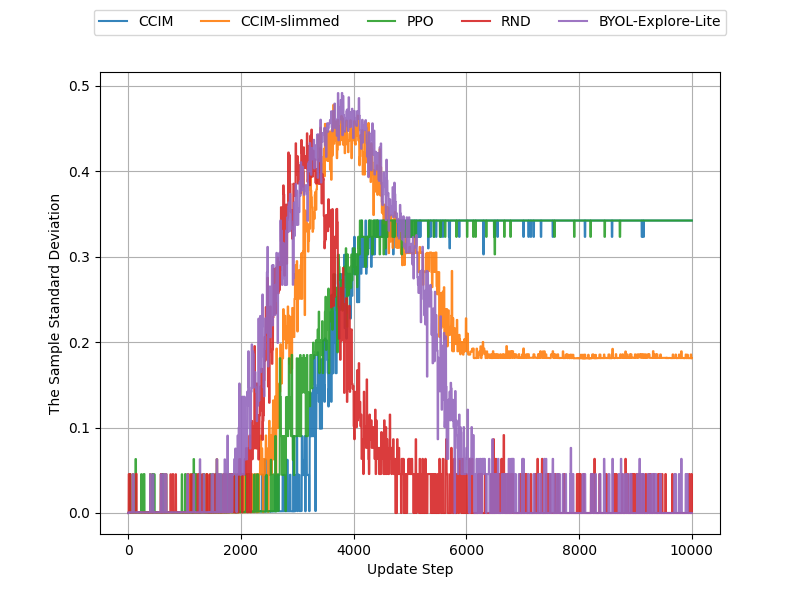
Each RL agent undergoes training for 500,000 time steps across four vectorized environments, employing 30 seeds for each RL algorithm. To assess performances on the environments, we calculate the average episode return across seeds at the end of training with a 95% confidence interval determined through the percentile bootstrapped method. We are not just interested in how well these curiosity algorithms perform but also in understanding the behaviour of these algorithms. We therefore also visualise the sample standard deviation during training to see the performance variations. This assists us in seeing how consistent the behaviour is for each curiosity algorithm and the normal PPO algorithm.
Now since we are not testing the reward combiner found, it is not clear how we should combine the external reward and the intrinsic reward. However, we treat both the external reward and the intrinsic reward as episodic and therefore we use the following formula, \(\hat{r} = r_t + \lambda ri_t\), where \(\lambda\) is some weight factor. These are the optimal values we found for \(\lambda\) for each curiosity algorithm:
- FAST: \(\lambda = 0.003\).
- CCIM-slimmed: \(\lambda = 0.17\).
- CCIM: \(\lambda = 0.003\).
- BYOL-Explore Lite: \(\lambda = 0.006\)
- RND: \(\lambda = 0.2\).
For FAST, CCIM, and CCIM-slimmed we normalise the intrinsic reward using the same method as RND. Next we describe the environments we use in more detail.
Empty grid-world
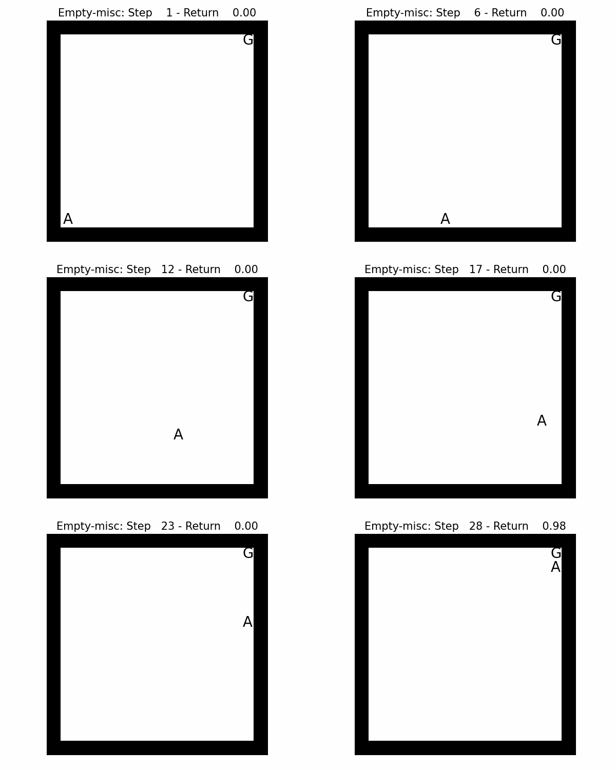
The empty grid-world is a very simple environment. As mentioned earlier the agent’s task is to reach the goal position. The size is \(16\times 16\) and the maximum number of steps is 1024. In our implementation the agent starts at the bottom left corner and has to reach the top right corner. The reward that agent recieves if it finds the goal is 1 - 0.9 * (step_count / max_steps). The gif shows a RL agent exploring the environment to reach the goal.
Deep sea
The deep sea environment is one of the bsuite environments developed by Google Deepmind
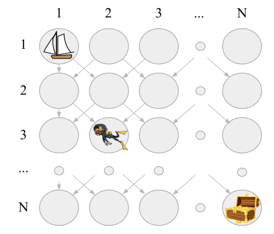
The agent starts at the top left corner and its goal is to reach the bottom right corner. At each time step the agent descends one row. The agent can either go left or right. There’s a small penalty of going right which is \(−0.01/N\) while going left just gives a reward of zero. The agent receives a reward of 1 if it finds the treasure at the bottom right corner. The max number of steps in the environment is \(N\). Therefore, the optimal policy is to go right at every time step ignoring the greedy action. In our experiments we set \(N=10\).
Results
CCIM
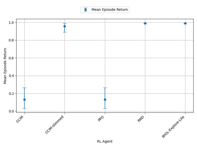
We start with the deep sea environment. The left of Figure 11 shows the sample standard deviation during training. We only show it for the first 10,000 steps because after that we notice the graphs plateau. We see that RND and BYOL-Explore Lite produce the most consistent agents in the deep sea environment. And CCIM-slimmed produces more consistent agents than CCIM and PPO. Looking at the right of Figure 11 we can see the mean episode return across the 30 seeds with the 95% confidence intervals. RND, BYOL-Explore, and CCIM-slimmed all perform better than PPO. However, CCIM does performs roughly the same as PPO at the end of training. From our experiments we also noticed that intrinsic rewards produced by CCIM increase and then plateau. The CCIM random and forward network’s loss continued to increase during training as well.
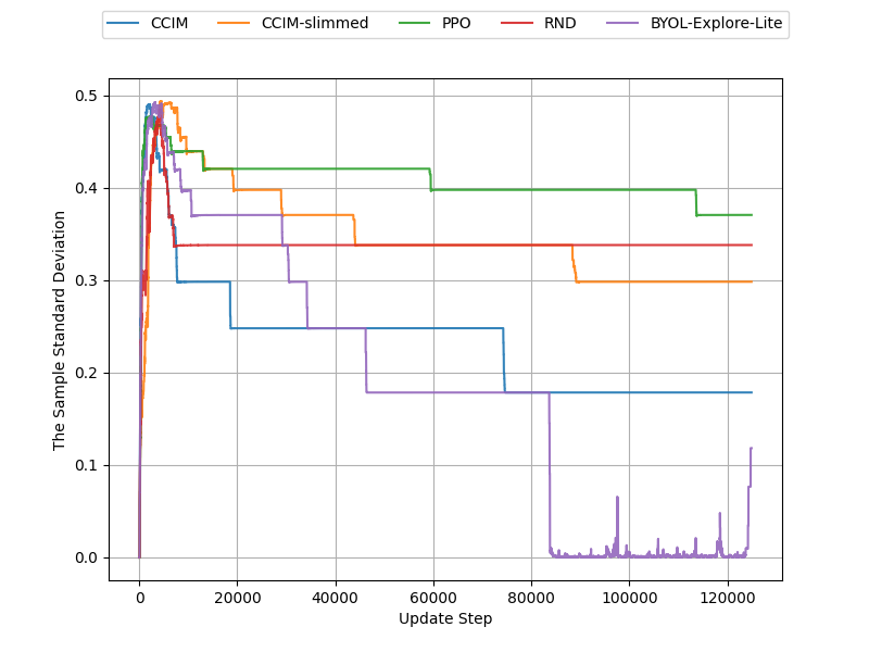
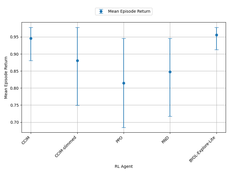
Next we move onto the empty grid-world. Looking at the left of Figure 12 we can see that all curiosity algorithms produce more consistent agents than PPO due to their sample standard deviations being lower. CCIM and CCIM-slimmed both actually produce more consistent agents than RND and PPO in this environment. The right of Figure 12 also indicate that CCIM performed much better in the empty grid-world and was closer to the baselines. However in this environment we did once again notice the raw intrinsic reward increased then plateaued and the loss of random forward network increased during training. It should also be noted the confidence intervals of all the RL algorithms overlap in the empty grid-world environment.
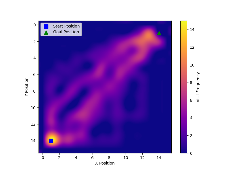
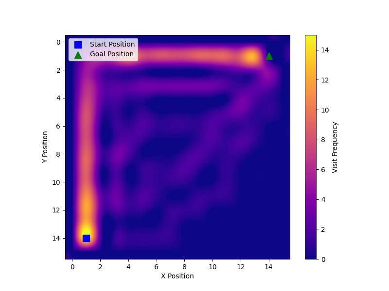
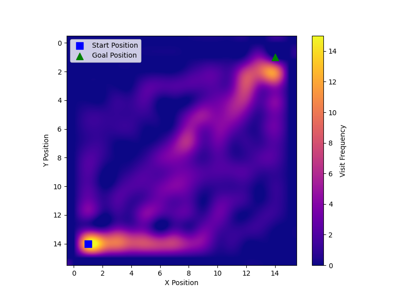
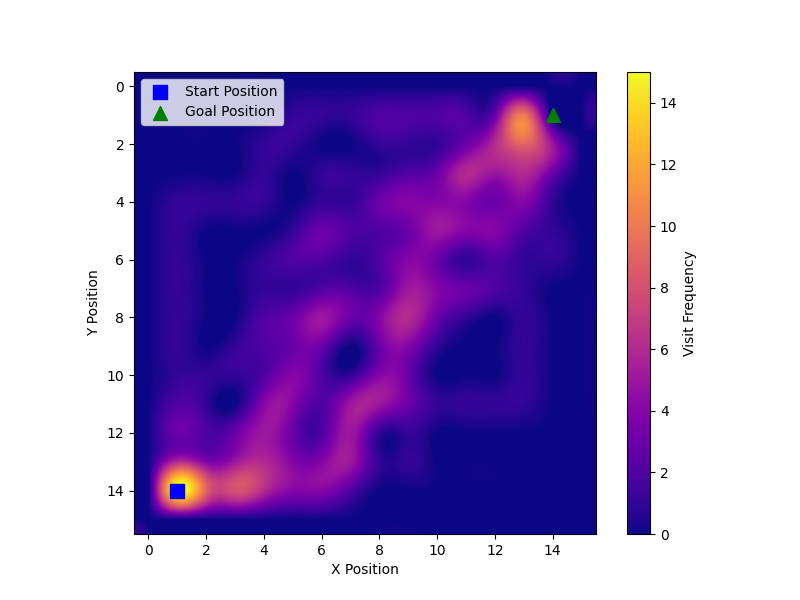
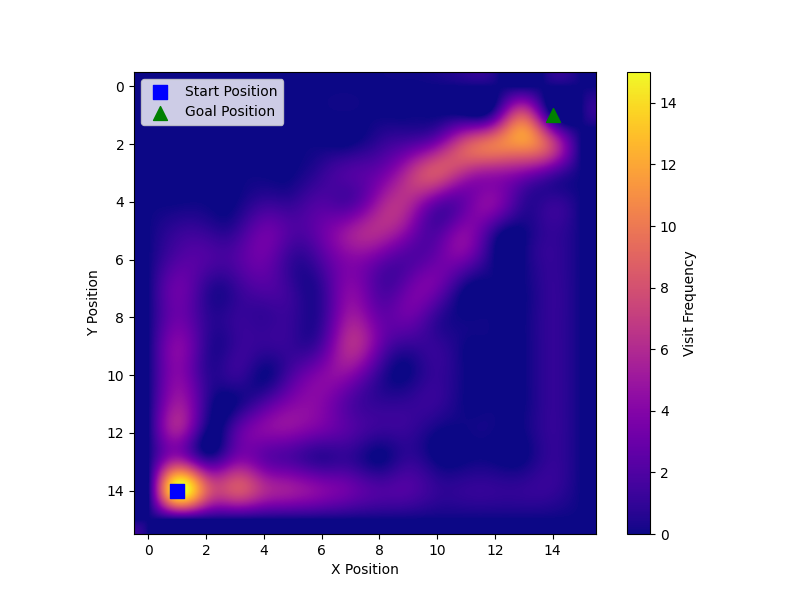
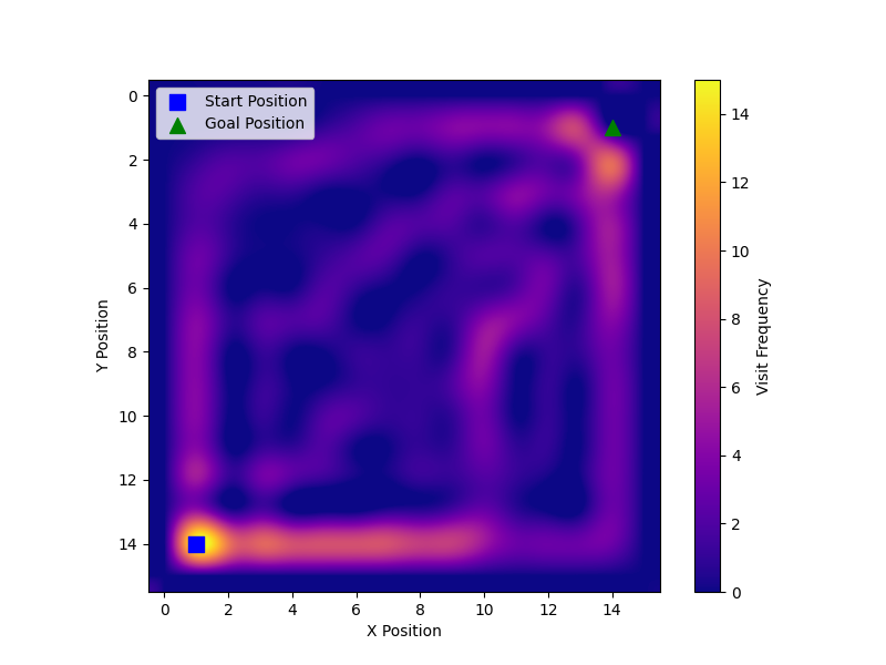
Next we decided to plot the RND, BYOL-Explore Lite, normal PPO, CCIM and CCIM-slimmed heatmaps in Figure 13 and 14. To make the heatmaps we looked at the best 15 seeds for each algorithm and kept track of the paths each seed took. Looking at Figure 13 and Figure 14, we can see that the CCIM and CCIM-slimmed covered more of the map than RND and BYOL-Explore Lite. However, they only covered slightly more of the map than PPO.
FAST
Let us now turn our attention to how FAST performed. We began with the deep sea environment. In Figure 15 we plot the sample deviation for the first 10,000 steps, as we observe no significant difference beyond this point. The left side of Figure 15 indicates that PPO and our curiosity-driven baselines produces more consistent agents than FAST as they exhibit a lower sample standard deviation.
On the right side of Figure 15, we see that FAST, similar to CCIM, performs poorly on this environment compared to our baselines. Notably, during training we noticed the intrinsic reward of the FAST agents also increased.
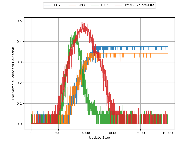
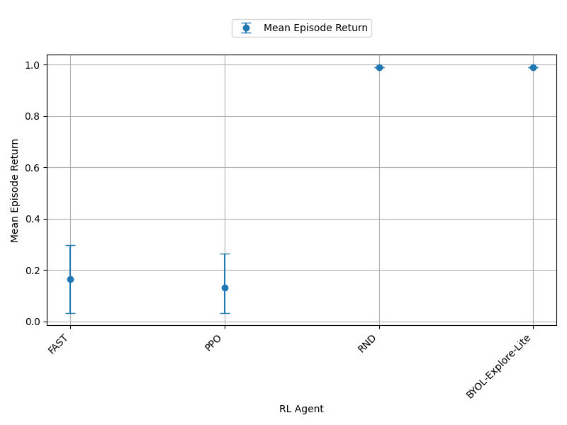
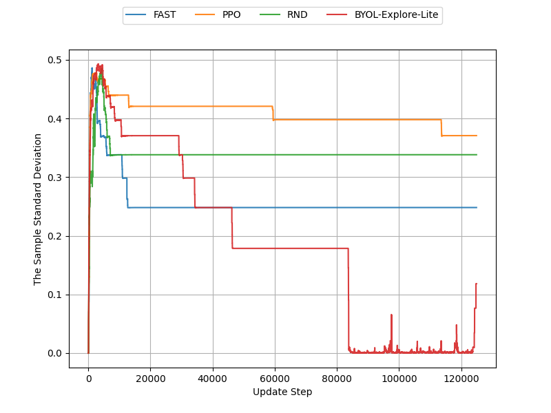
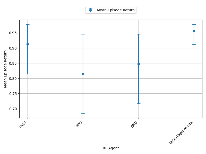
The right side of Figure 16 shows FAST’s performance in the empty grid-world is better than its performance in the deep sea environment; it is now comparable to our baselines despite its intrinsic rewards also increasing over time. Once again, similar to CCIM’s results, we observe overlapping confidence intervals in the empty grid-world. Figure 16 shows that not only has its performance improved in the empty grid-world but it now produces more consistent agents than RND and PPO as its sample standard deviation is lower.
We once again plot the heatmap of FAST and compare it to PPO’s heatmap using the best 15 seeds. When comparing Figure 17 (left) with both Figure 17 (right) and Figure 13, we observe that FAST covered more of the grid-world than PPO, BYOL-Explore Lite, and RND.

Discussion
Alet et al. provided a unique approach to meta-learning. The performance of CCIM and FAST in the empty grid-world then did not surprise us as that was the environment used to search for the algorithms. Note in Figure 17 that the 15 best seeds of FAST covered more of the map, i.e., most of the seeds took different parts to the goal compared to PPO. However for the CCIM and CCIM-slimmed heatmaps we notice that these algorithms only slightly covered more of the map then PPO. It should be noted that by looking at the heat maps that CCIM-slimmed, CCIM, and FAST both covered more of the map than our baselines which makes sense given Alet et al. looked for curiosity that optimise the number of distinct cells visited when searching for the curiosity algorithms.
From the sample deviation plots, we can see that FAST and CCIM do not produce consistent agents than PPO and the curiosity-driven baselines in the deep sea environment. While CCIM-slimmed produced more consistent agents than PPO but not the baselines. However, in the empty grid-world environment FAST, CCIM, and CCIM-slimmed is able to produce more consistent agents than PPO and RND. In the mean episode return plots, CCIM, CCIM-slimmed, and FAST perform better than PPO and RND in the empty grid-world environment which makes sense as the empty grid-world environment was used to find these curiosity algorithms. However, in the deep sea environment we see that the meta-learned curiosity algorithms perform worse than our curiosity-driven baselines.
From the mean episode return plots we can see that BYOL-Explore Lite is the best performing algorithm. Even in the empty grid-world environment it performs better than the meta-learned curiosity algorithms. We believe this is because of the reward prioritisation implemented in BYOL-Explore. This could explain its performance is better than the meta-learned curiosity algorithms and why it produces the most consistent agents.
One major concern we still have is how the intrinsic rewards for FAST and CCIM didn’t decrease during training for both environments used in our experiments. However, we noted that the intrinsic rewards for CCIM-slimmed decreased during training. We believe the decrease in intrinsic rewards as training progresses is one of the main reasons why BYOL-Explore and RND are effective and why we see the improved performance of the CCIM-slimmed algorithm. Even with the reward combiner, we still believe that the intrinsic rewards not decreasing could potentially cause an issue, as it did with the deep-sea environment.Recall that the reward combiner has the following formula,
\[\hat{r}_t = \frac{(1+ri_t-t/T)\cdot ri_t+ r_t\cdot t/T}{1+ri_t}.\]Now if \(t=T\) then the \(\hat{r}_t \approx r_t\) if \(0 \leq ri_t \ll 1\). However for us the intrinsic rewards were not much less than zero during training. We believe that it is important for curiosity algorithms that the intrinsic reward decreases as the agent becomes more familiar with its environment. We believe that this is why CCIM-slimmed performed better than CCIM and FAST in the deep sea environment. Another concern we have is how the CCIM random and forward network’s loss increased during training. It is possible that there’s a bug somewhere in our code which we have not found yet.
In the future we think it will be interesting to repeat this experiment using the deep sea environment to find the curiosity algorithms that output the intrinsic reward. Additionally, exploring the use of a variant of FAST or CCIM to find a reward combiner is also of interest to us. We wonder why a variant of FAST or CCIM wasn’t employed for this purpose, as a variant of RND was used to find the reward combiner. As stated earlier, FAST, CCIM and CCIM-slimmed do not make use reward prioritisation like BYOL-Explore Lite does. Therefore, repeating the experiments with the meta-learned curiosity algorithms where some form of reward prioritisation is implemented is another interesting path we hope to explore. We would also like to increase the number of seeds used to reduce the confidence intervals. Since we are training end-to-end in JAX in simple environments, increasing the number of seeds should not be much of an issue.
Conclusion
In this blog post, we studied two meta-learned curiosity algorithms, namely FAST and CCIM. We compared them to a non-curious agent and our baselines for the curiosity algorithms: RND and BYOL-Explore. Our experiments were conducted using both the empty grid-world environment and the deep-sea environment.
FAST and CCIM both performed well in the empty grid-world, covering more of the map than the baselines when examining their heatmaps. This aligns with our expectations since this was the environment used to search for the curiosity algorithms. However, in the deep-sea environment, both algorithms did not perform well compared to the baselines. Conversely, CCIM-slimmed, a slimmed down version of CCIM, showed performance comparable to the baselines. We suspect that this is because the intrinsic reward decreased as the agent explored more. This behaviour was not observed in FAST and CCIM, which we believe is not ideal and consider it the main flaw of these algorithms.
This approach of meta-learning curiosity algorithms is novel, and we believe there’s interesting work that can be done following the same approach as Alet et al., trying it with different environments to search for curiosity algorithms, such as the deep-sea environment. Moreover, BYOL-Explore makes use of reward prioritisation. Therefore, in the future, we hope to include reward prioritisation in our FAST, CCIM, and CCIM-slimmed implementations to see if it improves performance. Another avenue is using the meta-learned curiosity algorithms to search for the reward combiner.