Bridging the Parallel Decoding of LLMs with the Diffusion Process
In this blog, we introduce Jacobi Decoding, a parallel decoding algorithm for LLMs and its connection to the diffusion process in terms of high-level concepts. We propose that due to these structural similarities, many techniques developed for diffusion models hold tremendous potential for enhancing the decoding process of LLMs in the future.
Introduction
The decoding process of an autoregressive LLM involves the model generating text by predicting each token step-by-step from left to right. The core idea is to predict the next token based on the content generated so far, so each generated token updates the input, allowing the model to recursively use the previous output as the new input for the next prediction. Various decoding methods, such as greedy search and beam search, have been explored, with more detailed explanations available here. However, most of these methods aim to balance the stability and diversity of LLM outputs, sometimes introducing additional inference overhead. Moreover, since these decoding methods are inherently sequential, each decoding step does not leverage the parallel processing capabilities of modern GPUs, often resulting in low GPU utilization. This poses challenges for many real-world LLM applications that prioritize rapid response times, such as video understanding. In this blog, we will first introduce Jacobi Decoding, a parallel decoding method for autoregressive LLMs that aims to achieve faster decoding speeds with minimal performance drop. Secondly, we discuss the conceptual similarities between Jacobi Decoding and the diffusion process, which inspire us to borrow advantages from diffusion models to enhance the decoding process of LLMs. Lastly, we further elucidate how diffusion processes can address major drawbacks in autoregressive LLMs by showcasing several existing explorations.
Jacobi Decoding
Let’s start by defining some basic mathematical notation. For a general autoregressive LLM, we have:
\[y_i=\text{arg max}_y p(y|y_{;i},x)\]Here, \(x\) represents the input prompt, often referred to as the prefix, while \(y_{:i}\) denotes the tokens that have already been predicted, and \(y_i\) is the next token to be predicted. In this case, we simply select the token with the highest probability as the prediction for the next token.
The Jacobi iteration is a classic nonlinear system solver that, when applied to LLM decoding, can support generating multiple tokens at once rather than the traditional autoregressive one-at-a-time approach. Specifically, we first define the objective function:
\[f(y_i,y_{:i},x) = y_i -\text{arg max}_y p(y|y_{:i},x)\]We require that, for each position \(i\) in the decoded sequence, the condition \(f(y_i,y_{:i},x)=0\) holds. Simply put, this objective is equivalent to autoregressive decoding and serves as the upper bound for Jacobi Decoding. Assuming that the number of tokens decoded in one iteration is \(n\), the decoding process is equivalent to iteratively solving the following system of equations:
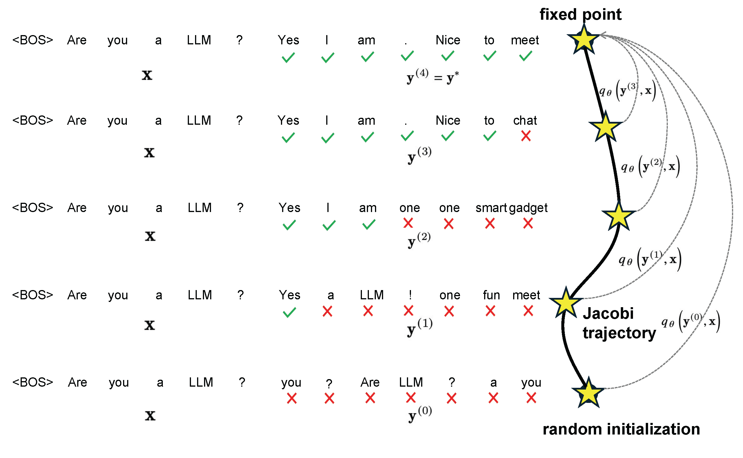
\[\begin{cases} y_1^{(j+1)}&=\text{arg max}_y p(y|x) \\ y_2^{(j+1)}&=\text{arg max}_y p(y|y_1^{(j)},x) \\ y_3^{(j+1)}&=\text{arg max}_y p(y|y_{:3}^{(j)},x) \\ &\vdots \\ y_n^{(j+1)}&=\text{arg max}_y p(y|y_{:n}^{(j)},x) \end{cases}\]Here, the superscript \(^{(j)}\) denotes the iteration count. It’s evident that each equation corresponds to standard autoregressive decoding. However, the difference lies in the dependency: while autoregressive decoding relies on precise preceding tokens, Jacobi Decoding solves for all tokens simultaneously, based on an imperfect initial guess. As illustrated in the following diagram, starting from a set of random guesses, the predicted sequence continually refines itself. Each iteration produces a more accurate sequence, which in turn yields even better predictions in the next iteration, ultimately converging to the autoregressive decoding result. The driving signal toward accuracy in this process is actually provided by the prefix \(x\).
Figure 1. Illustration of the parallel decoding process.

However, although these equations are mathematically in closed form, in practice, an LLM pre-trained in an autoregressive manner (based on precise preceding tokens) may not consistently achieve the same results when predicting with imprecise preceding tokens. Additionally, experiments have observed that even correctly predicted tokens are sometimes replaced in subsequent iterations, leading to unnecessary step wastage. Some works, such as Lookahead Decoding
Table 1. Comparison of parallel decoding strategies (Jacobi and lookahead) against AR decoding on finetuned models and CLLMs. Notably, CLLMs exhibit the ability of fast consistency generation while maintaining lower memory and computational demands.
| Methods | Speed (tokens/s) | Speedup | Metric | Size |
|---|---|---|---|---|
| Fine-tuned LlaMA2-7B | ||||
| + AR | 43.5 | 1.0x | 59.1 | 6.7B |
| + Jacobi | 45.7 | 1.1x | 59.1 | 6.7B |
| + lookahead | 74.8 | 1.7x | 59.1 | 6.7B |
| CLLM-LLaMA2-7B | ||||
| + AR | 43.5 | 1.0x | 56.4 | 6.7B |
| + Jacobi | 132.4 | 3.0x | 56.4 | 6.7B |
| + lookahead | 125.2 | 2.9x | 56.4 | 6.7B |
Figure 2. Comparison of Jacobi decoding against AR decoding.

Diffusion Process
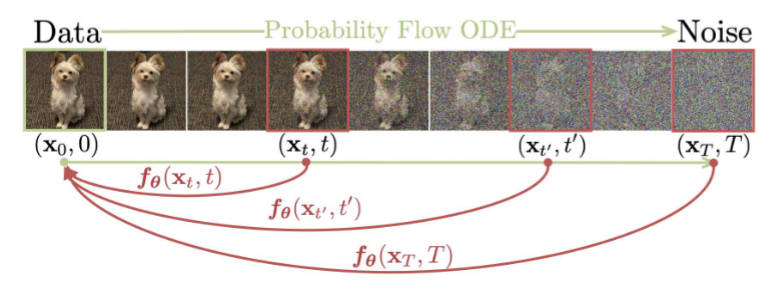
If we view each iteration of Jacobi Decoding as a state transition between tokens, it actually shares many formal similarities with discrete diffusion models. In CLLM
Figure 3. Diffusion process of consistency models.

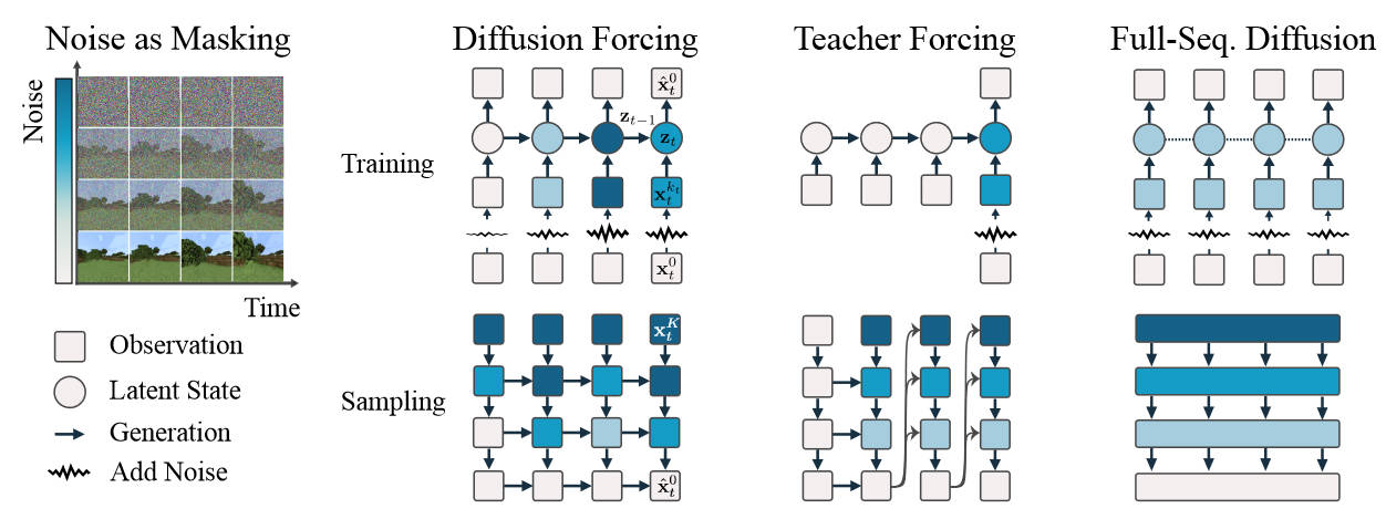
Due to these structural similarities, many techniques developed for diffusion models may be transferable to Jacobi Decoding in the future. For example, diffusion models perform sequence editing naturally by adding noise and then denoising, which could enable faster text editing, refinement, or style transfer based on Jacobi Decoding. When working with a longer input text, Jacobi Decoding could be significantly faster than in-context learning approaches in autoregressive decoding. Moreover, for editing tasks where a well-initialized token sequence is already available, Jacobi Decoding would likely be more stable than using random token initialization in text generation. Diffusion Forcing
Figure 4. Diffusion Forcing, a new training paradigm where a diffusion model is trained to denoise a set of tokens with independent per-token noise levels.

Existing Explorations
An exciting trend in current research is centered on combining large language models (LLMs) with diffusion processes. A series of studies have demonstrated the potential of diffusion language models (DLMs) in achieving controllable text generation, parallel text generation, and global planning, effectively addressing major drawbacks found in the autoregressive (AR) approach.
CLLMs: Consistency Large Language Models
The speedup effect of Jacobi decoding for vanilla LLMs is minimal in practice. The reason is that AR-trained LLMs can usually generate only one correct token in each Jacobi iteration as such models can rarely yield a correct token when there are incorrect preceding tokens. To address this, we propose to adapt pre-trained LLMs to consistently map any point \(y\) on the Jacobi trajectory $J$ to the fixed point \(y^∗\).
CLLMs is jointly optimized with two losses, one guaranteeing the prediction of multiple tokens at once and the other avoiding the CLLM from deviating from the target LLM so as to maintain generation quality.
Consistency Loss. For a prompt x with the Jacobi trajectory \(J\) , directly push CLLM to output \(y^∗\) with \(y\) as the input by minimizing the following loss:
\[\mathcal{L}_{GC} = \mathbb{E}_{(x, \mathcal{I}) \sim \mathcal{D}, y \sim \mathcal{I}} [ \sum_{i=1}^{n} D ( q_{\theta^-} (\cdot | y_{:i}^{*}, x) \| q_{\theta} (\cdot | y_{:i}, x) ) ]\]Alternatively, the adjacent states \(y(j), y(j+1)\) in the Jacobi trajectory J are demanded to yield the same outputs:
\[\mathcal{L}_{LC} = \mathbb{E}_{(x, \mathcal{I}) \sim \mathcal{D}, (y^{(j)}, y^{(j+1)}) \sim \mathcal{I}} [ \sum_{i=1}^{n} D ( q_{\theta^-} (\cdot | y_{:i}^{(j+1)}, x) \| q_{\theta} (\cdot | y_{:i}^{(j)}, x) ) ].\]AR Loss. To avoid deviating from the distribution of the target LLM, we incorporate the traditional AR loss based on the generation \(l\) of the target LLM \(p\):
\[\mathcal{L}_{AR} = \mathbb{E}_{(x, l) \sim \mathcal{D}} [ - \sum_{i=1}^{N} \log q_{\theta}(l_i \mid l_{:i}, x) ].\]The objective mentioned above is analogous to that of Consistency Models, as outlined by Song
Diffusion-LM Improves Controllable Text Generation
Diffusion-LM
Figure 5. A graphical model representing the forward and reverse diffusion processes. In addition to the original diffusion models, Diffusion-LM adds a Markov transition between \(x_0\) and \(w\).

The framework of Diffusion-LM is shown in Figure. To apply a continuous diffusion model to discrete text, Diffusion-LM adds a Markov transition from discrete words \(w\) to \(x_0\) in the forward process, parametrized by \(q(x_0,w) = \mathcal{N}(\text{EMB}(w), 0I)\). \(\text{EMB}(w_i)\) is an embedding function that maps each word to a vector in \(\mathbb{R}^d\). In the reverse process, Diffusion-LM rounds a predicted \(x_0\) back to discrete text by adding a trainable rounding step, parameterized by \(p_\theta(w,x_0) = \prod_{i=1}^n p_\theta(w_i,x_i)\), where \(p_\theta(w_i,x_i)\) is a softmax distribution. Rounding is achieved by choosing the most probable word for each position, according to \(\text{arg max} p_\theta(w,x_0) = \prod_{i=1}^n p_\theta(w_i,x_i)\). Ideally, this argmax-rounding would be sufficient to map back to discrete text, as the denoising steps should ensure that \(x_0\) lies exactly on the embedding of some word. The training objectives is:
\[\mathcal{L}_{\text{vlb}}^{e2e}(\mathbf{w}) = \mathbb{E}_{q_{\phi}(\mathbf{x}_0 | \mathbf{w})} [ \mathcal{L}_{\text{vlb}}(\mathbf{x}_0) + \log q_{\phi}(\mathbf{x}_0 | \mathbf{w}) - \log p_{\theta}(\mathbf{w} | \mathbf{x}_0) ],\] \[\mathcal{L}_{\text{simple}}^{e2e}(\mathbf{w}) = \mathbb{E}_{q_{\phi}(\mathbf{x}_0, \mathbf{x}_1 | \mathbf{w})} [ \mathcal{L}_{\text{simple}}(\mathbf{x}_0) + \| \text{Emb}(\mathbf{w}) - \mu_{\theta}(\mathbf{x}_1, 1) \|^2 - \log p_{\theta}(\mathbf{w} | \mathbf{x}_0) ].\]Controllable Text Generation. By performing control on the sequence of continuous latent variables \(x_{0:T}\) defined by Diffusion-LM, Controllable Text Generation can be achieved. Specifically, controlling \(x_{0:T}\) is equivalent to decoding from the posterior \(p(x_{0:T},c) = \prod_{t=1}^T p(x_{t-1},x_t, c)\), and we decompose this joint inference problem into a sequence of control problems at each diffusion step: \(p(x_{t-1},x_t, c) \propto p(x_{t-1},x_t) \cdot p(c,x_{t-1}, x_t)\). We further simplify \(p(c,x_{t-1}, x_t) = p(c,x_{t-1})\) via conditional independence assumptions from prior work on controlling diffusions. Consequently, for the \(t\)-th step, the gradient update on \(x_{t-1}\) is:
\[\nabla_{\mathbf{x}_{t-1}} \log p(\mathbf{x}_{t-1} \mid \mathbf{x}_t, \mathbf{c}) = \nabla_{\mathbf{x}_{t-1}} \log p(\mathbf{x}_{t-1} \mid \mathbf{x}_t) + \nabla_{\mathbf{x}_{t-1}} \log p(\mathbf{c} \mid \mathbf{x}_{t-1}).\]where both \(\log p(x_{t-1},x_t)\) and \(\log p(c,x_{t-1})\) are differentiable: the first term is parameterized by Diffusion-LM, and the second term is parameterized by a neural network classifier. Similar to work in the image setting, we train the classifier on the diffusion latent variables and run gradient updates on the latent space \(x_{t-1}\) to steer it towards fulfilling the control.
Beyond Autoregression: Discrete Diffusion For Complex Reasoning And Planning
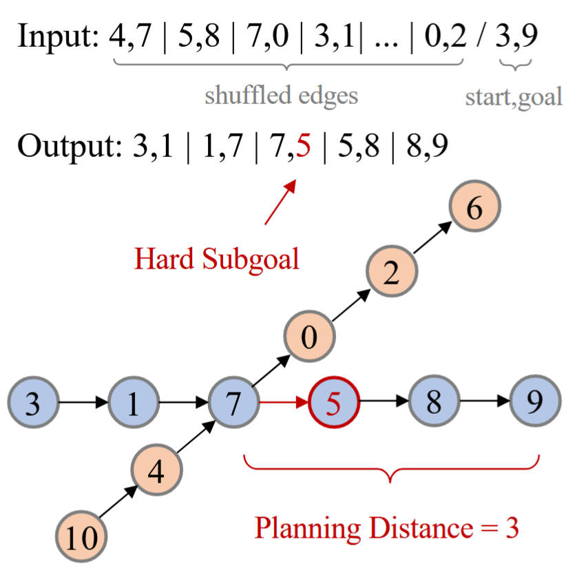
The generation of individual tokens may not inherently follow an autoregressive pattern. Consider the example in Figure, where the input for the task consists of a set of shuffled edges from the graph shown below. At the end of the input sequence, the start and goal nodes are specified to indicate the path the model needs to find. The objective of this task is to identify the correct path in the graph and output its constituent edges. The complexity of this problem arises from distracting factors (highlighted in orange) that potentially mislead the path selection. For instance, at node 7, with the goal being node 9, the model must plan over a distance of 3 nodes to determine that the correct next choice should be node 5 rather than 0. We define this span as the Planning Distance (PD), a parameter adjustable in our synthetic task data. Intuitively, as the PD increases, the model faces greater difficulty in learning to determine the correct subsequent node.
Figure 6. An illustration of the planning task.

Consequently, the difficulty of learning various subgoals can differ significantly. Given only the left context, some subgoals may require substantially more data to learn or may even be infeasible to learn. To address the issue of subgoal imbalance, this paper introduces multi-granularity diffusion modeling (MDM), which incorporates an additional token-level reweighting mechanism to enhance training efficiency:
\[L_{MDM} = \sum_{n=1}^{N} \sum_{t=1}^{T} w(t) v(\mathbf{x}_{t,n}) u(\mathbf{x}_0, \mathbf{x}_t, n; \boldsymbol{\theta}),\]where \(v(x_t,n)\) is the adaptive token-level reweighting term. Setting larger \(v(x_t,n)\) emphasizes harder tokens. This approach prioritizes different subgoals based on their difficulty during the learning process, leading to more effective learning outcomes and faster convergence.
Conclusion
As autoregressive models continue to dominate the landscape of language modeling, the exploration of alternative decoding methods remains a crucial area of research. Jacobi Decoding, recognized as a parallel decoding technique, presents a compelling strategy for enhancing the efficiency of large language models (LLMs). By harnessing the parallel processing capabilities inherent in GPUs, Jacobi Decoding can markedly accelerate the decoding process, rendering it more suitable for real-time applications. Furthermore, the relationship between Jacobi Decoding and the diffusion process offers novel insights that can inform the development of more efficient decoding methodologies for LLMs.