On LLM Knowledge Distillation - A Comparison between Forward KL and Reverse KL

In this blog post, we delve into knowledge distillation techniques for Large Language Models (LLMs), with a particular focus on using Kullback-Leibler (KL) Divergence as the optimization objective. Knowledge distillation is a powerful tool to reduce model size while maintaining comparable performance, making it especially useful in scenarios with constrained computational or serving resources. We specifically explore the nuances of Forward KL divergence and Reverse KL divergence, examining their roles in the distillation process. By comparing these two approaches, we aim to uncover their behaviours, strengths, and practical applications in LLM distillation.

Background

In recent years, knowledge distillation (KD) has gathered significant attention, particularly in the area of generative large language models (LLMs). Open-source LLMs, such as Qwen2 and LLaMA-3, come in a wide range of sizes, from 0.5 billion to 405 billion parameters. This diversity makes them ideal candidates for KD: training a high-performing model with a larger teacher model and subsequently distilling its knowledge into a smaller student model. This process is especially valuable when computational resources are constrained.

There are two primary approaches to knowledge distillation in LLMs:

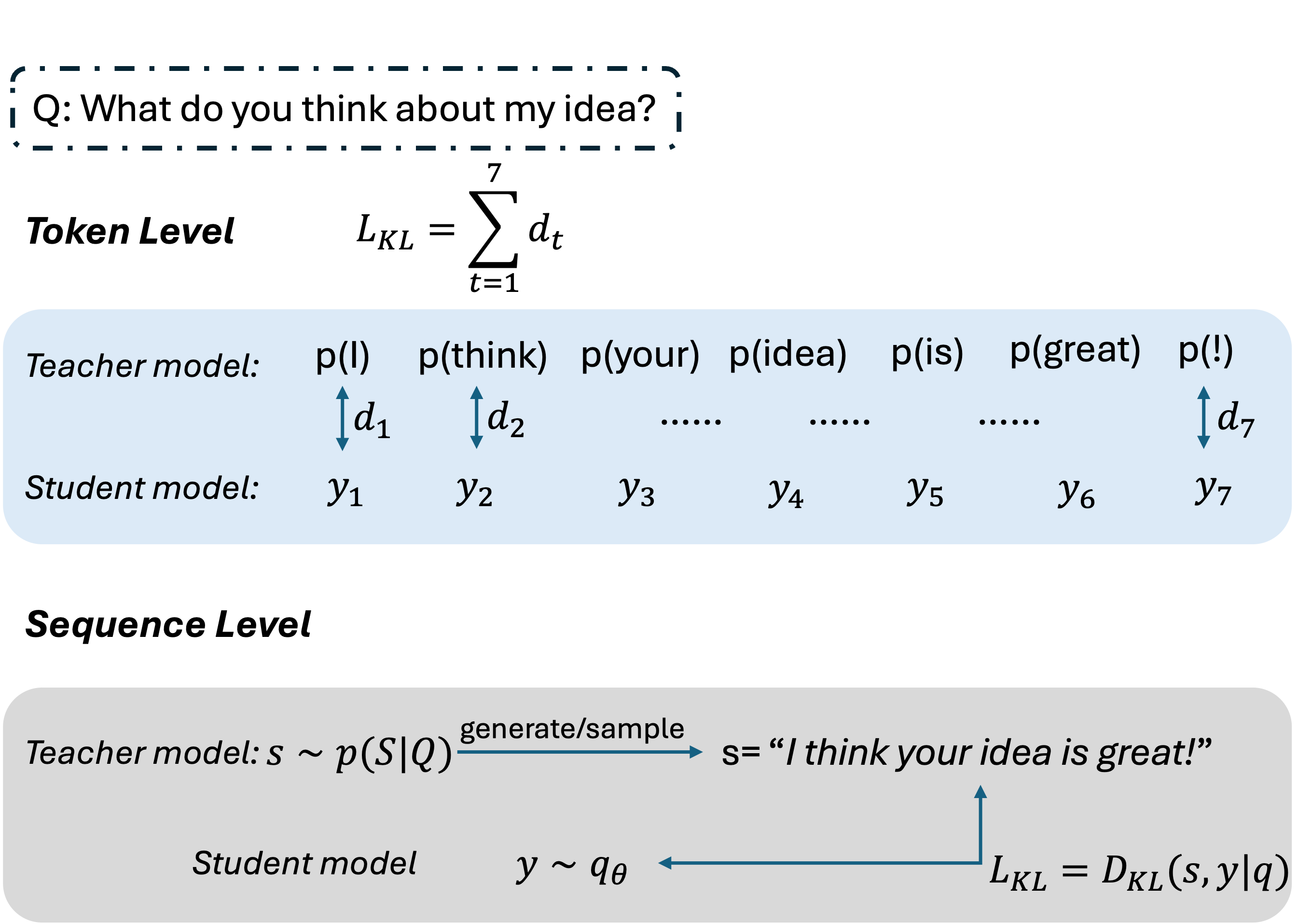
Sequence level distillation: This involves prompting the teacher model to generate responses, which are then used for distillation training. This approach is particularly effective when the teacher is a black-box system, accessible only via APIs.
Token level distillation: This approach aligns the intermediate outputs, such as logits or embeddings, between the teacher and student models. By focusing on token-level or layer-level alignment, it enables the distillation of deeper knowledge beyond the model’s final outputs.

In this blog post, we specifically focus on white-box knowledge distillation, which provides greater access to the teacher model’s internal representations and mechanisms. Unlike traditional knowledge distillation, which is primarily applied to classification-dominated tasks, knowledge distillation for modern generative language models presents unique challenges. For example, vanilla knowledge distillation using forward KL divergence as the loss function has been shown to introduce issues such as hallucination in language models. This could arise from forward KL’s inherent tendency toward mean-seeking optimization, which can lead to distorted or unrealistic outputs in generative tasks.

In this blog post, we will:

Provide an overview of knowledge distillation in generative language models, and the theoretical underpinnings of forward KL and reverse KL Divergence.
Review and analyze recent advancements in KD for LLMs, conducting an empirical comparison of methods.
Investigate forward KL divergence and reverse KL divergence fitting behaviour in detail.

By bridging these gaps, we aim to advance the understanding and application of KD in generative language modeling tasks.

Preliminaries

Knowledge Distillation in Conditional Language Modeling

Given a source-target pair (commonly referred to as an instruction-response) $(x,y)$, a language model $M$ is trained to accept the input $x$ and produce an output $\hat{y}=M(x)$, with the optimization objective being to minimize the discrepancy between $\hat{y}$ and $y$. Here, $x$, $y$, and $\hat{y}$ are sentences, and gradients are computed at the sentence level.

In the context of knowledge distillation for conditional language modeling, given an input source or instruction $x$, a teacher model generates a probability distribution $p(y\mid x)$, while a student model, parameterized by $\theta$, generates a distribution $q_\theta(y\mid x)$. The goal of knowledge distillation is to minimize the divergence between the teacher’s distribution $p(y\mid x)$ and the student’s distribution $q_\theta(y\mid x)$, enabling the student model to “mimic” the teacher’s behavior.

To ensure stable training, the distillation loss is typically combined with the supervised fine-tuning loss, allowing the student model to balance imitation of the teacher with alignment to ground truth data.

KL Divergence

The Kullback-Leibler (KL) divergence is a commonly used measure of the “distance” of two distributions. It can identity how far one distribution is to another. This is very useful in knowledge distillation cause the optimization goal we mentioned above is to make the student distribution similar enough to the teacher distribution. Using the denotes we have to formulate the KL divergence in knowledge distillation problems, given a student distribution (approximate distribution) $q_\theta(y\mid x)$ and a teacher distribution (true distribution) $p(y\mid x)$, the KL divergence can be formulated ashttps://dibyaghosh.com/blog/probability/kldivergence.html:

\[D_{KL}(p\|q_\theta)=\mathbb{E}_{y \sim p} \left[ \log \frac{p(y\mid x)}{q(y\mid x)} \right] \tag{1}\]

To be noticed, KL divergence is not a “symmetric” measure, which means that $D_{KL}(p|q_\theta)$ is not completely equal to $D_{KL}(q_\theta|p)$, even though the “meaning” is the same – how similar one distribution is to the other one.

Forward KL Divergence and Reverse KL Divergence

The difference between $D_{KL}(p|q_\theta)$ and $D_{KL}(q_\theta|p)$ becomes very prominent when using this KL divergence in optimization, i.e. minimizing the difference between two distributions. When we let student distribution to fit the real distribution, or the teacher distribution here, different order of $p$ and $q_\theta$ will result in difference in fitting performance, especially in the first several steps.

Suppose $D_{FKL}=D_{KL}(p|q_\theta)$ and $D_{RKL}=D_{KL}(q_\theta|p)$, where $D_{FKL}$ refers to forward KL divergence and $D_{RKL}$ refers to reverse KL divergence, the optimization goal can be formulated as:

\[\begin{aligned} \arg\min_{\theta} D_{FKL} &= \arg\min_{\theta} D_{KL}(p\|q_\theta) \\ &= \arg\min_{\theta} \mathbb{E}_{y \sim p} \left[ \log \frac{p(y|x)}{q_\theta(y|x)} \right] \\ &= \arg\max_{\theta} \mathbb{E}_{y \sim p} \left[ \log q_\theta(y|x) \right] \end{aligned} \tag{2}\]

and for reverse KL:

\[\begin{aligned} \arg\min_{\theta} D_{RKL} &= \arg\min_{\theta} D_{KL}(q_\theta \| p) \\ &= \arg\min_{\theta} \mathbb{E}_{y \sim q_\theta} \left[ \log \frac{q_\theta(y|x)}{p(y|x)} \right] \\ &= \arg\max_{\theta} \mathbb{E}_{y \sim q_\theta} \left[ \log p(y|x) \right] + \mathcal{H}(q_\theta(y|x)) \end{aligned} \tag{3}\]

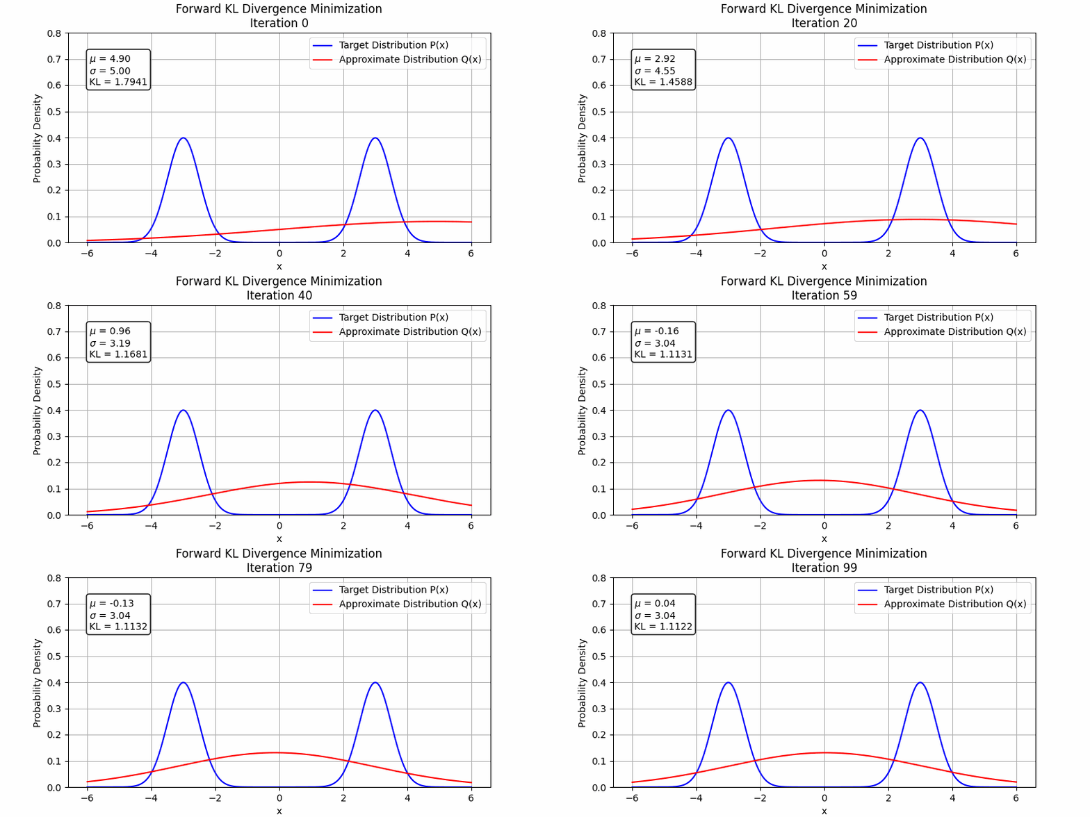
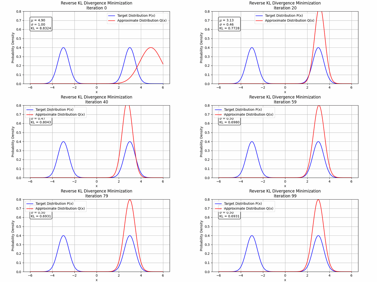
Forward KL is a mean-seeking behavior, while Reverse KL is a Mode-Seeking behavior https://dibyaghosh.com/blog/probability/kldivergence.html . This observation is often demonstrated by using one gaussian distribution to fit sum of two gaussian distributions. the fit progress could be found in the following figures.

Figure 1. One Gaussian distribution fitting sum of two Gaussian distributions.

To understand this phenomenon, $D_{FKL}$ represents the expectation calculated under the $p$ distribution, so it will match $q_\theta$ to $p$ where $p$ is high and the $q_\theta$ is low during the first steps, so $D_{FKL}$ will firstly increase $q_\theta$ where $q_\theta$ is low and $p$ is high. Under the condition of fitting two Gaussian distributions with one Gaussian distribution, the forward KL divergence will make the fitting distribution to be mean-seeking behavior

On the other hand, $D_{RKL}$ represents the expectation calculated under the $q_\theta$ distribution, so it will match $q_\theta$ to $p$ where $q_\theta$ is high and $p$ is low during the first steps, so $D_{RKL}$ will firstly decrease $q_\theta$ where $q_\theta$ is high and $p$ is low. Under the condition of fitting two Gaussian distributions with one Gaussian distribution, after reverse KL find a peak, it will stay at that Local optimum, which makes the fitting distribution to be mode-seeking behavior.

The behavior changes when a stronger student model is employed. In the following figures, we illustrate this by fitting the sum of two Gaussian distributions using sum of two Gaussian distributions. Both forward KL and reverse KL are capable of approximating the sum. Under these optimization settings, forward KL converges to a solution around step 100, while reverse KL achieves convergence around step 350. This suggests that with a sufficiently powerful student model and enough training steps, forward KL and reverse KL are likely to exhibit similar performance.

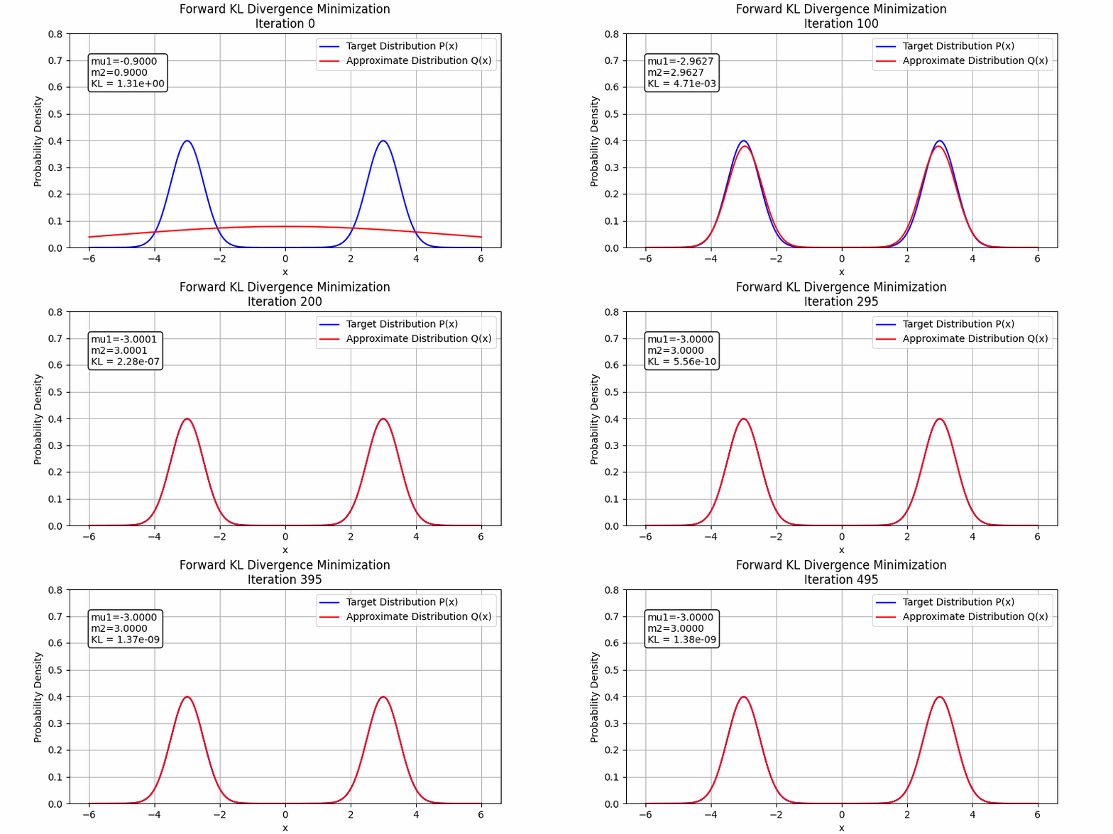
Figure 2. Two Gaussian distributions fitting sum of two Gaussian distributions

The detailed code to generate these images could be found in toy_example_fkl_rkl.py and toy_example_fkl_rkl_v2.py

Modern LLM Distillation Methods

To better suit knowledge distillation methods with modern large language model finetuning, multiple methods have been proposed. In this section, we summarize these methods from two levels, distillation from token level and from sequence (sentence) level.

As previously discussed, source/input $x$, output $\hat{y}$ and target $y$ are all sentences. During finetuning and knowledge distillation, the gradients can be applied to the general sentence, or the separated tokens. Here we denote $y=\{y_t\}_{t=1}^T$ where $y_t$ refers to the token at position $t$, and $T$ refers to the length of the sentence, i.e. number of tokens in $y$.

Figure 3. Illustration of token level knowledge distillation and sequence level knowledge distillation.

Modeling from Token Level

Most methods now are modeling the sentence distributions from token levels. By tokenizing the sentence $y$ into a sequence $\{y_t\}_{t=1}^T$, we can formulate the distillation optimization goal as:

\[\begin{aligned} \arg\min \mathcal{L}_{KL} &= \arg\min D_{KL}(p\|q_\theta) \\ &= \arg\min \sum_{t=1}^T D_{KL}( p( y_t \mid x,y_{1:t-1} ) \ \| \ q_{\theta}( y_t \mid x,y_{1:t-1} ) ) \end{aligned} \tag{4}\]

For token level knowledge distillation, the optimization goal per token is the same as the ones frequently used in embedding distillation, and computer vision. Forward KL divergence and reverse KL divergence are both commonly used loss functions in token level distillation. There’s no very clear observation or proof of which one would be a better choice for which case. Since the optimization goal is the same, the performance doesn’t seem to differ a lot when the model is fully trained. Sometimes both work, and inspired by this, some people begin to add the forward KL and reverse KL together. proposes Adaptive KL (AKL) divergence, which is an adaptive weighted sum of reverse KL and forward KL.

Modeling from Sequence Level

Different from token level distillation, sequence level distillation aims to let the student model match the teacher’s output probability over the whole sequence. For a generative model, it acquires knowledge by learning from the real-world distributions, which is natural language here. By performing Monte Carlo sampling from this distribution, the model generates sentences. From a token-level perspective, learning at each token position can be seen as a token classification task. However, from a sequence-level perspective, the entire sentence represents a sample drawn from the generative model’s learned distribution. This fundamental characteristic emphasizes a key distinction between sequence-level and token-level knowledge distillation in large language models. In sequence-level knowledge distillation, Monte Carlo sampling is typically used to draw samples that approximate the target distribution, capturing the sequence-level dynamics of the model’s behavior. This approach inherently differs from the token-level distillation process, where focus lies on individual token probabilities rather than the whole sequence.

From the perspective of implementation, the monte carlo sampling refers to model.generate. For a given input source, we can get two kinds of outputs from the model:

tokenized_inputs = tokenizer(**tokenized_inputs)
output_logits = model(**tokenized_inputs) # This is the logits/token level distribution.
output_sentence = model.generate(**tokenized_inputs) # This is the decoded/sampled sentence from the model.

where output_logits is the token level distribution, which is used to do token level distillation, and output_sentence is the sampled sequence, which is used in sequence level distillation.

Forward KL and Reverse KL are often employed in sequence-level knowledge distillation. The forward KL optimization goal can be formulated as:

\[\arg\min D_{KL}(p\|q_\theta)=\arg\min \mathbb{E}_{y\sim p}\log \frac{p(y\mid x)}{q_\theta(y\mid x)}\]

we can directly sample sentences $y from the teacher distribution. In simple terms, this optimization function lets the teacher model generate responses and uses the forward KL divergence as the loss function in knowledge distillation.

However, when the objective switches to reverse KL, i.e.,

\[\arg\min D_{KL}(q_\theta\|p)=\arg\min -\mathbb{E}_{y\sim q_\theta}\log \frac{(y\mid x)}{q_\theta(y\mid x)}\]

we need to sample from the student distribution. Since the student distribution is parameterized, it becomes infeasible to directly calculate the KL divergence for optimization, as in the case of forward KL. MiniLLMaddresses this challenge by approximating $D_{KL}(q_\theta|p)$ using policy gradient methods, making it possible to optimize effectively even under the reverse KL setup. GKD introduce Generalized Knowledge Distillation (GKD) to provide flexibility in choosing both the generation source (teacher model or student model) and the loss functions between the student and teacher.

Empirical Comparison, how it works and which one is better?

In this section, we present our empirical study on using forward KL and reverse KL for large language model distillation. We walk through the implementation of token-level knowledge distillation and common problems in knowledge distillation.

Experiment Details

We use a subset of 20,000 examples randomly sampled from HuggingFaceH4/ultrachat_200khttps://huggingface.co/datasets/HuggingFaceH4/ultrachat_200k dataset as sampled from real natural language distribution. For base models, we use Qwen2.5 series models as the training starting point. All experiments are completed using one node with 8 Nvidia A100 80G GPUs. Code and datasets will be released in [ADD GITHUB LINK HERE].

Implementation of Token-level Knowledge Distillation

In this section, we use forward KL as an simple example. For easy implementation and experimentation, we recommend using trl trainershttps://github.com/huggingface/trl and Huggingface alignment-handbookhttps://github.com/huggingface/alignment-handbook.

We inherits DistilTrainer from trl’s SFTTrainer, so that we don’t need to add some commonly used hyperparameters and functions. Similar implementation can be found in this code repo.

class DistilTrainer(SFTTrainer):
    def distillation_loss(self, student_logits, teacher_logits, inputs, original_loss):
        student_logits, teacher_logits = pad_logits(student_logits.to(self.model.device), teacher_logits.to(self.model.device))

        temperature = self.args.distillation_temperature
        alpha = self.args.distillation_alpha
        
        student_logits_scaled = student_logits / temperature
        teacher_logits_scaled = teacher_logits / temperature

        # Compute probabilities and log probabilities for both student and teacher
        student_log_probs = F.log_softmax(student_logits_scaled, dim=-1)
        teacher_log_probs = F.log_softmax(teacher_logits_scaled, dim=-1)
        student_probs = F.softmax(student_logits_scaled, dim=-1) # noqa

        loss_kd = F.kl_div(
            student_log_probs,
            teacher_log_probs,
            reduction='batchmean'
        ) * (temperature ** 2) / self.args.max_seq_length

        return alpha * loss_kd + (1 - alpha) * original_loss

Here we mainly emphasize the distillation loss. Given the student logits and teacher logits from model forward, we first pad the input logits into the same size. Then, we apply the given temperature to both logits. This softens the output distributions, making it easier for the student to learn. By using functions.kl_div , we can directly calculate the forward KL loss and add it together with the original cross entropy loss.

To address frequent out-of-memory (OOM) issues during distillation—caused by large tensor computations and the need to serve two models simultaneously—we strongly recommend leveraging the DeepSpeed strategies. Specifically, refer to the PPOTrainer example here and ensure _prepare_deepspeed is implemented accordingly to optimize resource utilization. If the teacher model is exceptionally large (e.g., a 64B parameter model), we suggest a two-step process: first, perform teacher model inference and save the resulting logits. Then, during training, load these precomputed logits to perform backpropagation. This approach significantly reduces memory requirements and streamlines the distillation process.

Empirical Study on Task-Agnostic Knowledge Distillation

Token-level Forward KL and Reverse KL

In this section, we present our experiment results on token-level forward KL and reverse KL in LLM knowledge distillation in the Table. All models are evaluated using the same eval set on ROUGE1, ROUGE2, ROUGEL and BARTScore. We continue using the above denotations, where $q_\theta$ refers to the parameterized student model, and $p$ refers to the teacher model. Except for distilled models, we also present the supervised finetuning results as baselines. All experiments settings are kept the same, which are available in code repo.

$q_\theta$	$p$	$q_\theta$ Size	$p$ Size	Loss	ROUGE1	ROUGE2	ROUGEL	BARTScore
Instruct	-	7B	-	-	0.4613	0.2059	0.2705	-2.5047
Ultra	-	1.5B	-	1.0*SFT	0.5295	0.2562	0.3414	-2.5242
Ultra	-	7B	-	1.0*SFT	0.5576	0.283	0.364	-2.4594
Instruct	Instruct	7B	1.5B	0.5SFT+0.5FKL	0.5369	0.2595	0.3435	-2.5134
Ultra	Instruct	7B	1.5B	0.5SFT+0.5FKL	0.5404	0.2615	0.3463	-2.5104
Ultra	Instruct	7B	1.5B	0.8SFT+0.2FKL	0.5292	0.2567	0.3406	-2.5235
Ultra	Instruct	7B	1.5B	0.5SFT+0.5RKL	0.5291	0.2558	0.3408	-2.5211

Table 1. Token level forward KL and reverse KL knowledge distillation results. Since the base model used here is Qwen2.5 family, we use Instruct to refer to Qwen2.5-instruct series models, for instance, Instruct 1.5B refers to Qwen2.5-1.5B-Instruct. Ultra refers to Qwen2.5-instruct models finetuned on the Ultrachat subset training set. For loss functions, SFT refers to supervised finetuning cross entropy loss, FKL refers to forward KL divergence loss, and RKL refers to reverse KL divergence loss.

From the above results, we can see that for token level, there’s not much difference between forward KL and reverse KL. By adding the supervised finetuning cross entropy loss, the general learning can be more stablized.

Convergence speed

Let’s begin the comparison with a simple task. Consider a single-layer fully connected network without bias, where both the input and output dimensions are 64. The network’s output is directly passed through a softmax layer.

We generated a fixed weight matrix with varying expected ranks and used this matrix as a fixed teacher model. Two student models with identical structures were trained, one guided by forward KL loss and the other by reverse KL loss.

Since forward KL loss and reverse KL loss differ in their formulations, their loss values are not directly comparable. Instead, we assess their convergence speeds using two proxy metrics: the L2 distance between the student and teacher probability distributions, and the L2 distance between the teacher’s weights and the student’s weights.

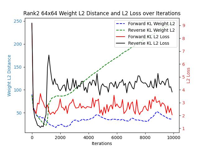
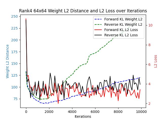
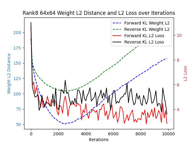
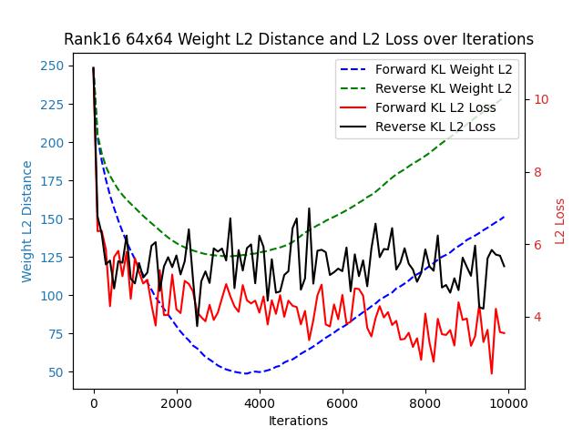
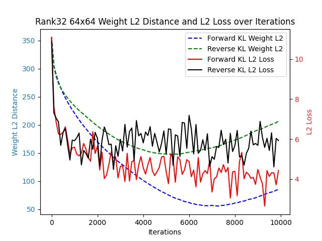
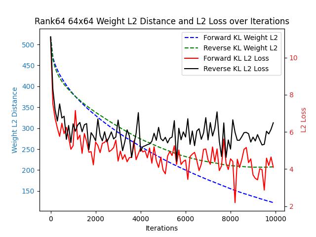
Figure 4. Convergence speed for Reverse KL and Forword KL.

Across all the images above, regardless of changes in the target matrix’s rank, forward KL consistently outperforms reverse KL in both weight-L2 and L2 loss.

Closing Remarks

In this blog post, we examined knowledge distillation techniques for Large Language Models (LLMs), specifically comparing Forward KL and Reverse KL Divergence. Our empirical results demonstrate that both divergence measures perform similarly at the token level, with Forward KL showing faster convergence in simple scenarios. However, the choice between Forward KL and Reverse KL may depend on specific model architectures and training conditions.

We also highlighted the challenges of applying knowledge distillation methods from computer vision to generative language models, emphasizing the need for specialized approaches in the context of LLMs. Future research could explore hybrid divergence strategies or adaptive weighting to further optimize distillation performance.

Effective knowledge distillation remains crucial for developing efficient LLMs that maintain high performance while reducing computational requirements. By continuing to refine these techniques, we can enable broader deployment of powerful language models in diverse applications.